Magnetic Dipole App

Magnetic Dipole App#

Now that we have learned how to interact with geoh5 and to create a custom user-interface with ui.json, we can start implementing our first application. We are going to create a a magnetic dipole simulator from scratch, which could become a useful tool to interpret magnetic data maps.

mag_dipole_gif

Background#

Python needs to import external libraries for certain classes and functions to be recognized when running the code. That is done below.

# Import the necessary packages
from __future__ import annotations

import json

import numpy as np
from geoh5py.data import Data
from geoh5py.objects import ObjectBase, Points
from geoh5py.ui_json import InputFile, constants, templates
from geoh5py.ui_json.utils import monitored_directory_copy
from geoh5py.workspace import Workspace

from training import assets_path

The physics#

The strength of the magnetic field flux of a single dipole is:

\[\mathbf{B} = \frac{\mu_0}{4 \pi} \left( \frac{3 \mathbf{r} (\mathbf{m} \cdot \mathbf{r})}{r^5} - \frac{\mathbf{m}}{r^3} \right)\]

where \(\mu_0\) is a constant (\(4 \pi \times 10^{-7}\)), \(\mathbf{m}\) is the magnetic dipole moment (susceptibility \(\times\) volume), and \(\mathbf{r}\) is the vector between the dipole and the locations.

In a geophysical context however, we normally get Total Magnetic Intensity (TMI) data from magnetometers. The conversion can be approximated by a projection of the fields onto the direction of Earth’s inducing field.

\[ b_{TMI} \approx \mathbf{\hat H}_0 \cdot \mathbf{b} \]

Arrays#

We will make use a few useful methods on numpy arrays.

The sum() method applied to a specific axis of an array, collapsing the dimension.
The dot() method performs the dot product between two arrays
The transpose (.T) method to get the dimensions of arrays to align:

\([1 \times 3] \cdot [M \times 3].T \rightarrow [1 \times M] \).

Array broadcasting (repeat) of a 1D array along a second dimension using the [:, None] indexing:

\([N \times 3] \;/\;([1 \times N][: None]) \rightarrow [N \times 3] \)

To-Do#

In order to compute the physics of dipoles, we will need:

Functions:
- Converting dip/azimuth angles to vector components
- Computing the fields of a dipole(s)
- Converting vector fields to TMI
Inputs parameters:
- Receivers (observation) locations
- Source dipole locations
- Dipole moment values
- Dipole inclination angles
- Dipole declination angles
- Earth’s field inclination
- Earth’s field declination

Functions#

Inclination / declination to vector conversion#

We require a function to convert inclination/declination angles to Cartesian vectors. The same function will come handy later when computing the TMI projection. We need to perform the following conversion:

\( \hat x = \sin(\phi) * \cos(\theta)\)

\( \hat y = \sin(\phi) * \sin(\theta) \)

\( \hat z = \cos(\phi) \)

where \(\phi\) is the angle on the horizontal plane, and \(\theta\) is the vertical angles. Both are positive counter-clockwise with reference from the \(\hat x\)-axis, so we also need to convert the angles from the geographic convention (degree clockwise from North).

def inclination_declination_2_xyz(inclination, declination):
    """Convert inclination and declination angles (degrees) to unit vector (xyz)."""
    theta = np.deg2rad((450 - declination) % 360)
    phi = np.deg2rad(90 + inclination)
    xyz = np.c_[np.sin(phi) * np.cos(theta), np.sin(phi) * np.sin(theta), np.cos(phi)]

    return xyz

Dipole functions#

We can begin with writing the function needed to compute the magnetic field from a single dipole.

\[\mathbf{B} = \frac{\mu_0}{4 \pi} \left( \frac{3 \mathbf{r} (\mathbf{m} \cdot \mathbf{r})}{r^5} - \frac{\mathbf{m}}{r^3} \right)\]

The function should be able to take as argument

- Coordinates of the source and receivers (defining 'r'),

- Parameters defining the strength (moment) and orientation (inc, dec) of the dipole source.

def b_field(source, locations, moment, inclination, declination):
    """
    Compute the magnetic field components of a dipole on an array of locations.

    :param source: Location of a point dipole, shape(1, 3).
    :param locations: Array of observation locations, shape(n, 3).
    :param moment: Dipole moment of the source (A.m^2)
    :param inclination: Dipole horizontal angle, clockwise from North
    :param declination: Dipole vertical angle from horizontal, positive down

    :return: Array of magnetic field components, shape(n, 3)
    """
    # Convert the inclination and declination to Cartesian vector
    m = moment * inclination_declination_2_xyz(inclination, declination)

    # Compute the radial components
    rad = source - locations

    # Compute |r|
    dist = np.sum(rad**2.0, axis=1) ** 0.5

    # mu_0 / 4 pi  * 1e9 for nT
    constant = 100
    fields = constant * (
        ((np.dot(m, rad.T).T * 3 * rad) / dist[:, None] ** 5) - (m / dist[:, None] ** 3)
    )

    return fields

We can now test our b_field function with existing objects present in our suncity.geoh5 project.

with Workspace(assets_path() / "suncity.geoh5") as workspace:
    # get variables
    source = workspace.get_entity("SunCityLocation")[0].vertices
    output_entity = workspace.get_entity("SunCity")[0]
    locations = output_entity.centroids
    m = 50**3 * 0.05 * 57000

    # compute fields
    field = b_field(source, locations, m, -67, -17)

    # write back to workspace
    output_entity.add_data(
        {
            "bx": {"values": field[:, 0]},
            "by": {"values": field[:, 1]},
            "bz": {"values": field[:, 2]},
        }
    )

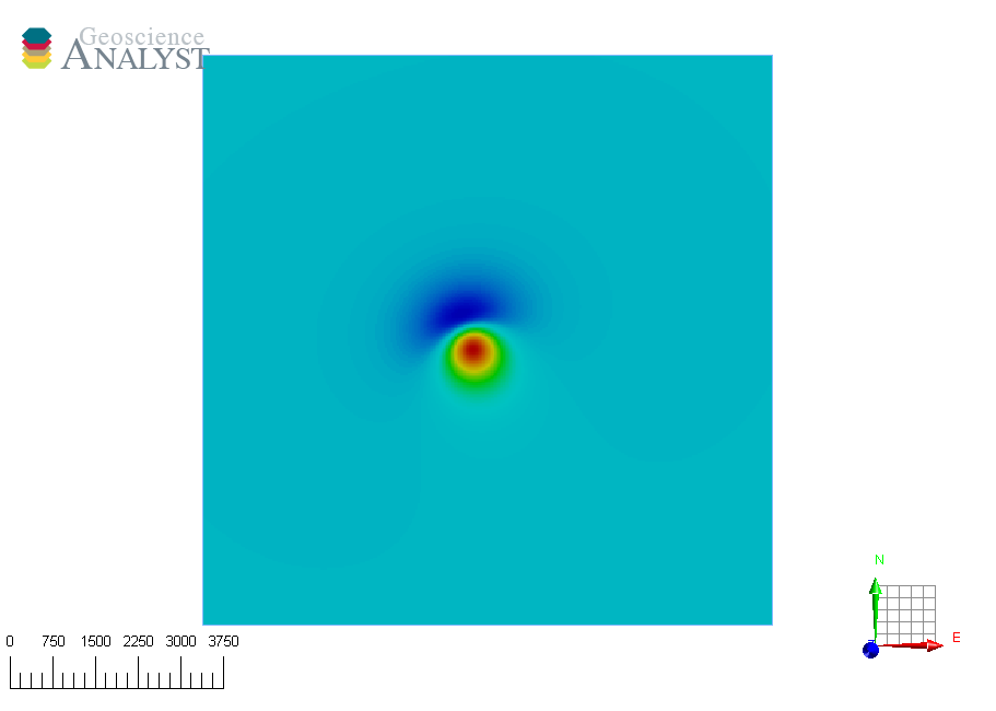
The b_field function returns an array for the three components of the magnetic field due to the dipole source.

TMI projection#

Let’s write a simple function to get the TMI (projected) data instead.

\[ b_{TMI} \approx \mathbf{\hat H}_0 \cdot \mathbf{b} \]

def tmi_projection(b_components, earth_field):
    """Project magnetic field onto Earth's field."""
    h0 = inclination_declination_2_xyz(earth_field[0], earth_field[1])
    return np.dot(h0, b_components.T)

and test it for the inducing field parameters at our test site at Suncity (Inc: -62.11, Dec: -17.9).

with Workspace(assets_path() / "suncity.geoh5") as workspace:
    # get variables
    source = workspace.get_entity("SunCityLocation")[0].vertices
    output_entity = workspace.get_entity("SunCity")[0]
    locations = output_entity.centroids
    m = 50**3 * 0.05 * 57000

    # compute fields
    earth_field = np.array([-45, 0])
    field = b_field(source, locations, m, earth_field[0], earth_field[1])
    tmi = tmi_projection(field, earth_field)

    # write back to workspace
    output_entity.add_data({"tmi_45": {"values": tmi}})

/home/docs/checkouts/readthedocs.org/user_builds/mirageoscience-python-training/conda/release-0.1.0/lib/python3.10/site-packages/geoh5py/data/numeric_data.py:114: UserWarning: Input 'values' converted to a 1D array.
  warn("Input 'values' converted to a 1D array.")

The Simulator#

In this section, we are going to string together the functions defined above and generalize our approach so that we can deal with different types of geoh5 objects. Let’s wrap all the previous functions into a magnetic_simulator class.

def magnetic_simulator(
    sources: ObjectBase,
    receivers: ObjectBase,
    moments: Data | float,
    inclinations: Data | float,
    declinations: Data | float,
    earth_inc: float,
    earth_dec: float,
):
    """
    Compute the magnetic field components of dipoles on a geoh5py object.

    :param sources: Points object of dipole locations.
    :param receivers: Array or Points object of observation locations.
    :param moments: Value or Data of dipole moments.
    :param inclinations: Value or Data of dipole inclination angles.
    :param declinations: Value or Data of dipole declination angles.
    :param earth_inc: Earth's field inclination angle.
    :param earth_dec: Earth's field declination angle.

    :return b_field: List of Data entities.
    """

    def locations(entity):
        if hasattr(entity, "centroids"):
            return entity.centroids

        return entity.vertices

    # Extract dipole coordinates
    dipoles = locations(sources)

    # Extract receiver coordinates
    observations = locations(receivers)

    def vectorize(entity):
        if isinstance(entity, Data):
            return entity.values

        return np.ones(dipoles.shape[0]) * entity

    # Get dipole moment values
    mom = vectorize(moments)
    # Get dipole inclination values
    inc = vectorize(inclinations)
    # Get dipole declination values
    dec = vectorize(declinations)

    # Loop over the dipoles
    fields = np.zeros_like(observations)

    for source, moment, inclination, declination in zip(dipoles, mom, inc, dec):
        fields += b_field(source, observations, moment, inclination, declination)

    tmi = tmi_projection(fields, (earth_inc, earth_dec))

    # Add data to receiver object
    data = receivers.add_data(
        {
            "b_x": {"values": fields[:, 0]},
            "b_y": {"values": fields[:, 1]},
            "b_z": {"values": fields[:, 2]},
            "tmi": {"values": tmi},
        }
    )

    return data

We now have a generic container to compute TMI data based on any type of ANALYST object.

You are now invited to edit your Points object to add more vertices and create data arrays for moment, azimuth and dips. We can now run the simulation by simply giving those entities to our class.

with Workspace(assets_path() / "suncity.geoh5") as workspace:
    # get variables
    source = workspace.get_entity("SunCityLocation")[0]
    output_entity = workspace.get_entity("SunCity")[0]

    m = 50**3 * 0.05 * 57000

    #
    data = magnetic_simulator(source, output_entity, m, -67, -17, -67, -17)
    print(data)

[<geoh5py.data.float_data.FloatData object at 0x7f4ebd3ec6a0>, <geoh5py.data.float_data.FloatData object at 0x7f4ebd39f8b0>, <geoh5py.data.float_data.FloatData object at 0x7f4ebd39f9a0>, <geoh5py.data.float_data.FloatData object at 0x7f4ebd39e980>]

bfield

The User-Interface (ui.json)#

In the previous section, we have introduced functionality to compute the magnetic field from dipole locations. We are now going to create a user-interface (UI) to be able to run this program from a Geoscience ANALYST session. Review the UIjson section for background.

We need a ui.json to provide inputs for the following 7 parameters:

Object defining the dipoles (sources)
Object defining the receivers
Data or float value for the dipole moments
Data or float value for the dipole inclination angles
Data or float value for the dipole declination angles
Float value for Earth’s field inclination angle
Float value for Earth’s field declination angle

Let’s create a UI.json with forms for each one of those inputs

mag_ui = constants.default_ui_json.copy()
mag_ui["title"] = "Magnetic Dipole App"
mag_ui.update(
    {
        "sources": templates.object_parameter(label="Dipoles", mesh_type="", value=""),
        "receivers": templates.object_parameter(
            label="Receivers", mesh_type="", value=""
        ),
        "moments": templates.data_parameter(
            label="Dipole Moment", parent="sources", value=1.0
        ),
        "inclination": templates.data_parameter(
            label="Dipole Inclination", parent="sources", value=-62.11
        ),
        "declination": templates.data_parameter(
            label="Dipole Declination", parent="sources", value=-17.9
        ),
        "earth_inc": templates.float_parameter(
            label="Earth's field Inclination", value=-62.11
        ),
        "earth_dec": templates.float_parameter(
            label="Earth's field Declination", value=-17.9
        ),
    }
)


# Some modifications
for label in ["moments", "inclination", "declination"]:
    mag_ui[label]["isValue"] = True
    mag_ui[label]["property"] = ""

We now need tell which “program” that ANALYST can call.

mag_ui["conda_environment"] = "python-training"
mag_ui["run_command"] = "mag_dipole_app"

Internally, when executed from ANALYST, this is what is going to happen

conda activate python-training
python mag_dipole

Then your mag_dipole.run should be able to do the rest: compute and store the result.

Let’s write out our ui.json to file.

with open(assets_path() / "magnetic_dipole.ui.json", "w", encoding="utf-8") as file:
    json.dump(mag_ui, file, indent=4)

Try running the UI through ANALYST with a drag & drop of the file to the viewport.

dragdrop

The Driver (Running with Geoscience ANALYST)#

In the previous section, we created our simulation program and a user-interface using the UI json format. As a final step, we need to define a driver program that can be called from ANALYST.

We are going to take advantage of the geoh5py.ui_json.InputFile class to handle value conversions between geoh5 and python, as well as the monitored_directory_copy function to handle the live link with ANALYST.

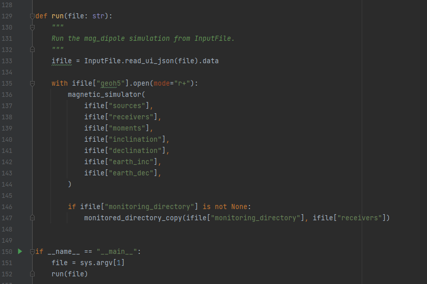
def run(file: str):
    """
    Run the mag_dipole simulation from InputFile.
    """
    ifile = InputFile.read_ui_json(file).data

    with ifile["geoh5"].open(mode="r+"):
        magnetic_simulator(
            ifile["sources"],
            ifile["receivers"],
            ifile["moments"],
            ifile["inclination"],
            ifile["declination"],
            ifile["earth_inc"],
            ifile["earth_dec"],
        )

        if ifile["monitoring_directory"] is not None:
            monitored_directory_copy(ifile["monitoring_directory"], ifile["receivers"])

The final step requires to make this program available to python to be executed from ANALYST.

Do the following:

Use the File\Download as\Python *.py dropdown menu to convert this notebook to a py file.
Rename the file to mag_dipole_app.py.
Remove everything in the file except the
- the imports,
- the blocks of functions def
- the following lines (without #’s)
```
if __name__ == "__main__":
    file = sys.argv[1]
    run(file)
```

This part becomes the entry point of the python interpreter when running the mag_dipole_app.py script. At the end, your file should look like this.

run_command

Executing in ANALYST#

We now have everything we need to run our program with custom user-interface. The last step consists in moving our ui.json and py file to ANALYST Script Directory. After re-opening of the workspace, your program will be visible in the drop-down menu.

uijson_add

Et voila!